PV-RCNN: Point-Voxel Feature Set Abstraction for 3D Object Detection

Last updated Jul 17, 2022 Edit Source

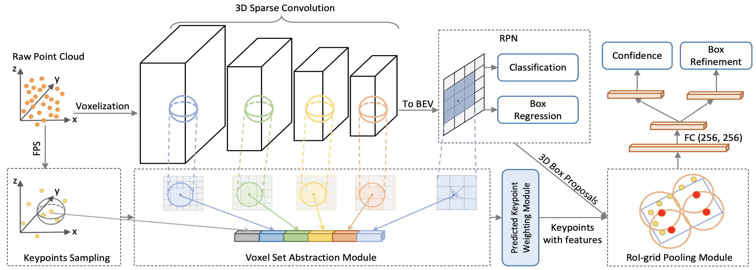
• Two stage detector that uses the point AND voxel features (via sparse convolution)
• Two novel operations:
  • Voxel-to-keypoint scene encoding:
    • which summarizes all the voxels of the overall scene feature volumes into a small number of feature keypoints
  • point-to-grid RoI feature abstraction:
    • effectively aggregates the scene keypoint features to RoI grids for proposal confidence prediction and location refinement

• Input points P are split into voxels $L\times W \times H$ in $(x,y,z)$ respectively.
• A $3\times 3 \times 3$ (3D) kernel is used in the sparse convulation.
  • result: P into feature volumes with $1\times,2\times,4\times,8\times$ downsampled sizes.
    • $2\times$ means the voxel size (or $L/W/H$?) is $2\times$ larger, so there are few voxels.
• One we have the the $8\times$ downsampled feature volumes $\left(\frac{L}{8}\times \frac{W}{8}\times \frac{H}{8}\right)$
  • we stack the voxels along the $Z$ axis to get a $\frac{L}{8}\times \frac{W}{8}$ bird-view feature maps.
  • what is stacking here
• Each class has $2\times \frac{L}{8} \times \frac{W}{8}$ 3D anchor boxes, and two anchors of $0^\circ$ and $90^\circ$ orientations. each anchor box is evaluated for each pixel of the BEV feature map.

• from P, we first use [FPS](notes/papers/PointNet++#Sampling Layer ) to sample $n$ keypoints $\mathcal{K}={p_1,\ldots,p_n}$
• Denote: $$\mathcal{F}^{(l_k)}={f_1^{(l_k)},\ldots,f_{N_k}^{(l_k)}}: \text{set of voxel-wise feature vectors at in }k\text{th level}$$ $$\mathcal{V}^{(l_k)}={v_1^{(l_k)},\ldots,v_{N_k}^{(l_k)}}: \text{set o}$$
• Where $N_k$ is the number of non-empty voxels in the $k$th level

For each keypoint $p_i$ we find neighboarding non-empty voxels at the $k$th level within radius $r_k$. The resulting set of voxel-wise features vectors is:$$S_{i}^{(l_k)}= \left { [f_j^{(lk)};\underbrace{v{j}^{(l_k)}- p_i}{\text{relative coords}}]^T ; \middle | ; \begin{array}{cc} \lVert v{j}^{(l_k)}-p_i \rVert^2 < r_{k}, \[1ex] \forall v_{j}^{(l_k)}\in \mathcal{V}^{(l_k)}, \[1ex] \forall f{j}^{(l_k)}\in\mathcal{F}^{(l_k)} \end{array} \right}$$ where:

• $v_{j}^{(l_k)}-p_i$ : relative coordinates/location of $f_j^{(l_k)}$

• $f_j^{(l_k)}$: semantic voxel feature

• The voxel-wise features within neighboring voxel set $S_{i}^{(l_k)}$ is then passed into a PointNet block:$$f_{i}^{(pv_k)}=\max\left{G\left(\mathcal{M}\left(S_{i}^{(l_k)}\right)\right)\right}\tag{2}$$

• where:

• $M(\cdot)$: randomly sampling at most $T_k$ voxels from $S_{i}^{(l_k)}$. (for saving computation)

• $G(\cdot)$: MLP

• $\max(\cdot)$: max-pooling along channel dimension.

  • The result of the block are the features of key point $p_i$

Then for each keypoint $p_i$ , we concatinate its features from different levels $$f_i^{(pv)}=\left[f_{i}^{(pv_1)},f_{i}^{(pv_2)},f_{i}^{(pv_3)},f_{i}^{(pv_4)}\right], \text{for } i=1,\ldots,n$$ where:

• $f_i^{(pv)}$: is 3D voxel CNN-based feature + pointnet features as explained above

• With the 8x downsampled 2D BEV feature map, and original point cloud P, put P through eq 2. We call these features $f_i^{(raw)}$
• Also project each $p_i$ onto the BEV map, and use bilinear interpolation to get $f_i^{(bev)}$ from BEV feature map
  • How exactly?
• Then finally concatinate all these features together:$$f_i^{(p)}=\left[f_{i}^{(pv)},f_i^{(raw)},f_{i}^{(bev)}\right], \text{ for }i=1,\ldots,n$$

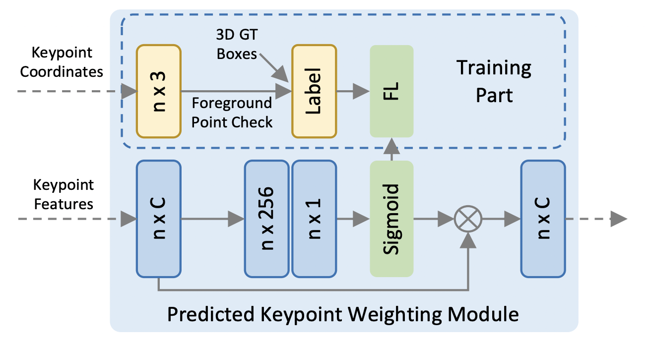
• Because [FPS](notes/papers/PointNet++#Sampling Layer) might chose background points, we want to put more weight into the foreground points + their features.
• Take the keypoint features, and pass it through a three layer mlp: $\mathcal{A}(f_i^{(p)})$ with sigmoid as the final layer as illustrated above.
  • In training this is supervised via checking if the keypoint is in a GT box or not. i.e.: $p_i$ has label $1$ if $p_i$ in GT, else $0$. Focal loss is used here.
• weights are then multiplied by the features: $$\tilde{f_i}^{(p)}=\mathcal{A}(f_i^{(p)})\cdot f_{i}^{(p)}$$

• After all the previous steps, we have the set of keypoint features $$\tilde{\mathcal{F}}=\left{\tilde{f_{i}}^{(p)},\ldots,\tilde{f_{n}}^{(p)}\right}$$
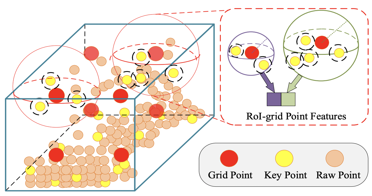
• For each 3D proposal (RoI) we need to aggregate the keypoint features
• We uniformly sample $6\times6\times6$ grid points within each 3D proposal (RoI) denoted as $\mathcal{G}={g_1,\ldots,g_{216}}$
  • (Grid points need not be points from raw pointcloud P)
• For each grid point, we gather all key point features within radius $\tilde{r}$ $$\tilde{\Psi}=\left{\left[\tilde{f}{j}^{(p)};p_j-g_i\right]^T ;\middle|; \begin{array}{@{}l@{}} \lVert p{j}-g_i\rVert^2 < \tilde{r}, \[1ex] \forall p_{j}\in \mathcal{K}, \[1ex] \forall \tilde{f}_{j}^{(p)}\in\tilde{\mathcal{F}} \end{array}\right}$$
• $p_j-g_i$: local coordinates of features $\tilde{f_j}^{(p)}$ relative to grid point $g_i$
• pointnet is used again to aggregate features: $$\tilde{f}_i^{(g)}=\max\left{G\left(\mathcal{M}\left(\tilde{\Psi}\right)\right)\right}$$
• Two seperate MLP heads (256 dims) are then used for box refinement and confidence.
  • Box Refinement: for each of the RoI, it predicts the residuals compared to GT. $$L_{iou}=-y_k\log(\tilde{y}_k)-(1-y_k)\log(1-\tilde{y}_k)$$
    • where $\tilde{y}_k$ is predicted score by network
  • Confidence: For the $k$th RoI, its confidence for a target $y_k$ is normalized to be between $[0,1]$ $$y_k=\min(1,\max(0,2\text{IoU}_k-0.5))$$
    • Where $\text{IoU}_k$ is the IoU of the $k$th RoI w.r.t to tis GT box.
  • Both are optimized via smooth-L1

• 3 Losses are used:
  • Region proposal loss: $L_{rpn}$ $$L_{rpn}=\underbrace{L_{cls}}{\text{focal loss}}+\beta \sum{r\in{x,y,z,l,w,h,\theta}}\mathcal{L}{smooth-L1}(\underbrace{\widehat{\Delta r^a}}{\substack{\text{predicted} \\ \text{residual}}},\Delta r^a)$$
    • predicted residual: $\widehat{\Delta r^a}$
    • regression target: $\Delta r^a$
  • Keypoint segmentation loss: $L_{seg}$
    • loss calculation is explained in the [Predicted Keypoint Weighting](notes/papers/PVRCNN#Predicted Keypoint Weighting)
  • Proposal refinement loss: $L_{rcnn}$ $$L_{rcnn}=L_{iou}+\sum_{r\in{x,y,z,l,w,h,\theta}}\mathcal{L}{smooth-L1}(\underbrace{\widehat{\Delta r^p}}{\substack{\text{predicted} \\ \text{residual}}},\Delta r^p)$$
    • predicted box residual: $\widehat{\Delta r^p}$
    • proposal regression target: $\Delta r^p$
• Overall loss is sum of these three with equal loss weights.