Supervised Learning
# What is supervised learning?
- Training an algorithm to output $y$ for a given $x$ using sufficient training samples ${(x^{(0)},y^{(0)}),(x^{(1)},y^{(1)}),\ldots,(x^{(n)},y^{(n)})}$ for some input $x^{(i)}$ and correct output $y^{(i)}$
- Regression: predicting an a number (infinitely many outputs)
- Classification: predicting categories (finite outputs)
# Linear Regression
- Given a training set we can use a learning algorithm to learnign a function $f$ that predicts an output $\hat{y}$ given an input $x$
- for linear regression, $f$ is a straight line. With parameters $w,b$ we can then represent $f$ as: $$f_{w,b}(x)=wx+b$$
# Cost Function
- Since our objective to find $w,b$ such taht $\hat{y}^{(i)}$ is close to $y^{(i)}$ for all $(x^{(i)},y^{(i)})$.
- Squared error cost function: $$J(w,b)=\frac{1}{2m}\sum^{m}_{i=1}(\hat{y}^{(i)}-y^{(i)})^2$$
- where $m=$ number of training examples. So $\frac{1}{m}$ is to average it so it doesnt blow up, factor of $2$ is for computational convience later.
- Now we can also rewrite it as: $$J(w,b)=\frac{1}{2m}\sum^{m}{i=1}f{w,b}(x^{(i)})-y^{(i)})^2$$
- This can be solved analytically for simple cost functions, but for complicated $J$, we can use gradiant descent to minimize $J$ instead:
# Gradient Descent
initialize $w,b$, calcuated $J$
adjust $w,b$ to decrease $J$
repeat until hopefully $J$ settles near minimum
Step 1: ($=$ here is assignment, not equals) $$w=w -\alpha \frac{d}{dw}J(w,b)$$ where $\alpha$ is the learning rate, a hyperparameter that controls the “fast” we change $w$
Step 2: do the same for $b$ $$b=b -\alpha \frac{d}{db}J(w,b)$$
Note: $w$ and $b$ must be updated at the same time.
# Learning rate
- If $\alpha$ is too small, then it will take many steps to reach minimum
- If $\alpha$ is too large, then it might never reach the minimum
# Gradient Descent for linear regression
Calculating derivatives for $w$, $$\frac{d}{dw}J(w,b)= \frac{d}{dw}\frac{1}{2m}\sum^{m}{i=1}(\hat{y}^{(i)}-y^{(i)})^2$$$$=\frac{d}{dw}\frac{1}{2m}\sum^{m}{i=1}(wx^{(i)}+b-y^{(i)})^2$$ which is equal to $$\frac{1}{m}\sum^{m}{i=1}(f{w,b}(x^{(i)}-y^{(i)})x^{(i)}$$
and derivative for $b$, $$\frac{d}{db}J(w,b)= \frac{d}{dw}\frac{1}{2m}\sum^{m}{i=1}(\hat{y}^{(i)}-y^{(i)})^2$$$$ =\frac{d}{db}\frac{1}{2m}\sum^{m}{i=1}(wx^{(i)}+b-y^{(i)})^2$$ which is equal to $$\frac{1}{m}\sum^{m}{i=1}(f{w,b}(x^{(i)})-y^{(i)})$$
Psuedocode for gradient descent:
| |
where dJdW = $\frac{d}{dw}J(w,b)$ and dJdb = $\frac{d}{db}J(w,b)$
# Multiple features
what if you have multiple features (variables)?
- $x_j = j^{th}$ feature
- $n$ = number of features
- $\vec{x}^{(i)}$= features of $i^{th}$ training example
- $x_{j}^{(i)}$ = value of feature $j$ in the $i^{th}$ training example
We can then express the linear regression model as:
$$f_{w,b}(x)=w_1x_1+w_2x_2+\cdots+w_nx_n+b$$ define $\vec{w} = [w_1,\ldots,w_n]$ and $\vec{x}=[x_1,\ldots x_n]^T$, $T$ here represents transpose. Then $$f_{\vec{w},b}=\vec{w}\cdot \vec{x}+b$$Where $(\cdot)$ represents the dot product.
# Feature Scaling
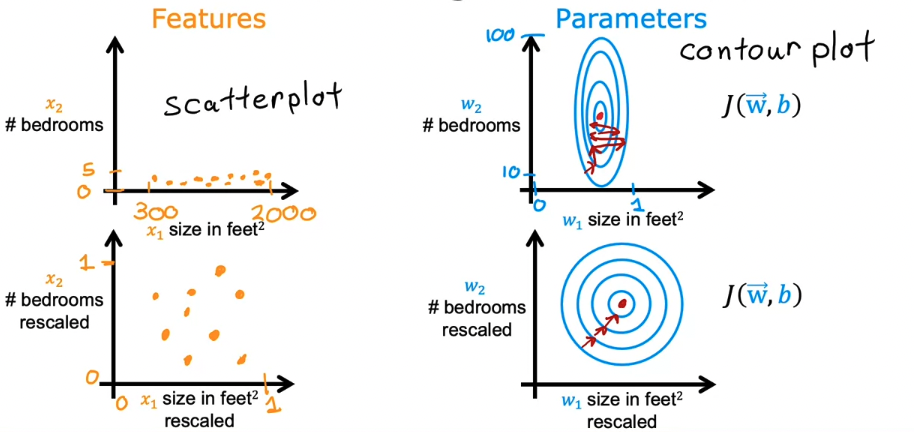
When the range of values your features can take up differ greatly, i.e.
- $x_1$ = square footage of house $\in [500,5000]$
- $x_2$ = number of bedrooms $\in [1,5]$
this may cause gradient descent to run slowly. 
Some examples of feature scaling
# max scaling
- divide each data point for a feature by the max value for that feature.
# mean normalization
- eg: if $300 \leq x_1 \leq 2000$ , we can scale it like such $$x_{1new} = \frac{x_1-\mu_1}{2000-300}$$
- where $\mu_1$ = mean
# Z-score normalization
- find standard deviation $\sigma$ , mean $\mu$ then $$x_1=\frac{x_1-\mu_1}{\sigma_1}$$